Summary

In this blog, we explore how AWS Bedrock foundational models perform under various load conditions and introduce a reusable testing methodology to help you understand performance characteristics in your own applications. Our findings reveal that prompt size significantly impacts scaling patterns, with large prompts degrading performance more rapidly as concurrency increases compared to smaller prompts. We demonstrate how performance testing connects abstract quota values to real-world capacity planning, helping build stronger cases for quota increase requests when needed.

Introduction: Why Performance Testing Matters

When integrating Large Language Models (LLMs) into production systems—particularly those served on managed services like AWS Bedrock—understanding performance characteristics is critical for both technical and business success. Performance testing becomes even more crucial when considering the service quotas that AWS imposes on Bedrock usage.

What This Blog Aims to Accomplish

In this blog, we set out to accomplish several key objectives:

• Establish a reusable methodologyfor performance testing AWS Bedrock foundation models that can be adapted for different use cases
• Develop a robust testing frameworkusing Python’s asynchronous capabilities to simulate real-world load patterns
• Measure and analyze critical performance metrics—particularly tokens-per-second, concurrency levels, and response times
• Provide actionable insightsinto how models behave under various load conditions
• Demonstrate how to visualize performance datato make informed scaling decisions
• Show how performance testing supports quota managementand helps build cases for quota increase requests

By sharing our approach and findings, we aim to help better understand the performance characteristics of AWS Bedrock models and make informed decisions when designing their applications.

AWS Bedrock Quotas and Their Impact

AWS accounts have default quotas for Amazon Bedrock that restrict how many requests you can make within specific timeframes. These quotas directly affect your application’s scalability and user experience.

Key service quotas for Amazon Bedrock include:

• Tokens Per Minute (TPM): Controls the total token throughput across your account
• Requests Per Minute (RPM): Limits the number of API calls you can make

These quotas apply specifically to on-demand inference and represent the combined usage across Converse, ConverseStream, InvokeModel, and InvokeModelWithResponseStream APIs for each foundation model, AWS Region, and AWS account. Note that batch inference operates under separate service quotas. For more information about how these quotas work, refer to Quotas for Amazon Bedrock.

Awareness of these quotas is crucial when designing your application architecture. If your usage requirements exceed the default quotas assigned to your AWS account, you’ll need to request an increase—a process that requires justification. For guidance on scaling with Amazon Bedrock, refer to Scaling with Amazon Bedrock.

Translating Abstract Quotas into Real-World Capacity

One of the biggest challenges with AWS Bedrock quotas is translating abstract metrics like TPM and RPM into practical application capacity. What do these numbers actually mean for your specific use case?

Performance testing helps answer critical questions like:

• User capacity: How many concurrent users can your quota actually support?
• A 10,000 TPM quota might support 100 users making complex requests or 500 users making simple ones
• Response throughput: What’s the actual token generation speed under different load patterns?
• Understanding how tokens-per-second scales with concurrent requests reveals your true throughput capacity
• Latency implications: How does approaching quota limits affect user experience?
• Testing reveals whether you’ll face gradual performance degradation or sudden failures as you approach limits
• Real-world usage patterns: How do your specific prompts and response lengths translate to quota consumption?
• A 5,000-token prompt with a 500-token response has very different quota implications than a 500-token prompt with a 5,000-token response

By conducting targeted performance tests with your actual prompts and expected usage patterns, you can translate abstract quota values into concrete capacity planning: “With our current quota, we can support X concurrent users with Y second response times.”

Performance testing is not merely a technical exercise—it’s a strategic necessity when deploying LLM applications on AWS Bedrock. By establishing a systematic approach to measuring and analyzing model performance under various load conditions, you gain critical insights that inform everything from architectural decisions to capacity planning and quota management.

Let’s now explore how to implement this testing methodology in practice, examining the code, metrics, and visualization techniques that will give you deep insights into your model’s performance characteristics.

Methodology: Building a Robust Testing Framework

Before diving into specific test results, it’s essential to understand how we approached the challenge of systematically testing AWS Bedrock models. Our methodology prioritizes reproducibility, controlled variables, and realistic simulation of production conditions. By creating a structured framework rather than ad-hoc testing, we can derive meaningful insights that translate directly to production environments.

• Test Runner (run_all_tests): Main orchestration function managing concurrent request scheduling
• Request Handler (call_chat): Wraps API calls with precise timing measurements
• Concurrency Monitor: Tracks active request counts throughout testing
• Data Collector: Aggregates performance metrics
• Visualization System: Generates insights from collected data

This modular design allows us to isolate each component for optimization and debugging while maintaining a cohesive testing approach.

Testing Modes

The framework supports two distinct testing approaches:

Sequential Mode

In this mode, each batch of concurrent requests fully completes before the next batch starts. This approach provides clean, isolated measurements without interference between batches, making it ideal for:

• Establishing baseline performance characteristics
• Measuring the system’s response to specific concurrency levels in isolation
• Creating reproducible benchmarks for comparing different configurations
• Determining the maximum throughput at various concurrency levels

Interval Mode

In this more realistic mode, new batches of requests launch at fixed intervals regardless of whether previous batches have completed. This approach better simulates real-world traffic patterns where:

• New user requests arrive continuously at varying intervals
• Earlier requests may still be processing when new ones arrive
• The system must handle fluctuating concurrency levels
• Resource contention between requests reveals system bottlenecks

This dual-mode approach allows us to both establish clear performance baselines (Sequential) and observe how the system behaves under more realistic load conditions (Interval).

Thread Pool Configuration

The testing framework needs to handle many concurrent requests without becoming a bottleneck itself. We configure a thread pool with sufficient capacity using Python’s ThreadPoolExecutor as shown below:

custom_executor = ThreadPoolExecutor(max_workers)

loop = asyncio.get_running_loop()

loop.set_default_executor(custom_executor)

This provides sufficient capacity to handle hundreds of concurrent requests without the testing framework itself becoming a bottleneck. The framework is designed to be configurable, allowing you to test different concurrency levels, request patterns, and model configurations with consistent methodology.

Request Handling Implementation

The core of our testing framework is the call_chat function, which handles individual API calls to AWS Bedrock while tracking precise timing metrics:

async def call_chat(chat, prompt):

“””

Increments the counter, records the start time, makes a synchronous API call in a separate thread,

then records the end time and decrements the counter before returning the parsed result

with the request start and end times added.

“””

global active_invoke_calls

async with active_invoke_lock:

active_invoke_calls += 1

try:

# Record the start time before calling the API.

request_start = datetime.now()

result = await asyncio.to_thread(chat.invoke_stream_parsed, prompt)

# Record the end time after the call completes.

request_end = datetime.now()

 

# Add the start and end times to the result.

result[‘request_start’] = request_start.isoformat()

result[‘request_end’] = request_end.isoformat()

return result

finally:

async with active_invoke_lock:

active_invoke_calls -= 1

This function provides several critical capabilities:

• Tracks concurrent call counts accurately using atomic operations
• Captures precise timing information for performance analysis
• Runs API calls in separate threads to avoid blocking the event loop
• Associates metadata with each request to enable detailed analysis

Test Orchestration

Our run_all_tests function serves as the orchestrator for the entire testing process:

async def run_all_tests(

chat,

prompt,

n_runs=60,

num_calls=40,

use_logger=True,

schedule_mode=”interval”,

batch_interval=1.0

):

# Implementation handles scheduling based on the selected mode

# Collects and processes results

# Returns structured data for analysis

The run_all_tests launches multiple batches of calls according to the specified schedule mode:

• In “interval” mode, it schedules a new batch every batch_intervalseconds regardless of whether previous batches have completed. This simulates real-world traffic patterns where requests arrive continuously.
• In “sequential” mode, it waits for each batch to complete before launching the next. This helps establish clear performance baselines without interference between batches.

By maintaining this unified orchestration approach, we ensure consistent testing methodology across different models and configurations, enabling valid comparisons.

Understanding Key Performance Metrics

To effectively evaluate LLM performance, you need to track the right metrics. This section explores the essential metrics that provide meaningful insights into your AWS Bedrock models’ performance characteristics.

When evaluating foundation models, several metrics are particularly relevant:

• Input Tokens: Number of tokens in the prompt
• Output Tokens: Number of tokens generated by the model
• Time to First Token (TTFT): Delay before receiving the first response token—critical for perceived responsiveness
• Time to Last Token (TTLT): Total time until complete response is received
• Time per Output Token (TPOT): Average time to generate each token after the first
• Tokens per Second (TPS): Throughput measure showing token generation rate
• Active Concurrent Calls: Number of requests being processed simultaneously

These metrics are collected for each request and then aggregated for analysis.

To calculate tokens-per-second (TPS), we use the inverse of time per output token:

tokens_per_second = 1/time_per_output_token

The TPS determine how many tokens the model can generate per second. Higher values indicate faster generation speeds.

Our framework automatically calculates statistical distributions for these metrics, allowing you to understand not just average performance but also variance and outliers:

tps_metric = “tokens_per_second”

mean_val = df[tps_metric].mean()

median_val = df[tps_metric].median()

min_val = df[tps_metric].min()

max_val = df[tps_metric].max()

These summary statistics reveal the stability and consistency of your model’s performance. A large gap between mean and median might indicate skewed performance, while high variance between minimum and maximum values suggests unstable performance.

Visualizing Performance Data

Raw data alone isn’t enough to derive actionable insights from performance tests. Effective visualization techniques transform complex performance patterns into easily understood visual representations that highlight trends, anomalies, and optimization opportunities.
Our framework includes specialized visualization functions that provide multiple perspectives on performance data:

Comprehensive Metrics Dashboard

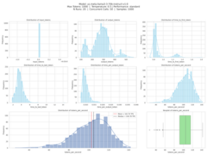
The plot_all_metrics function creates a consolidated dashboard with multiple visualizations:

def plot_all_metrics(df, n_runs, metrics=None):

“””

Creates one figure with 8 subplots using a subplot_mosaic layout “ABC;DEF;GGI”:

– 6 histograms/kde for the given metrics (A-F).

– 1 histogram/kde for tokens_per_second specifically (G).

– 1 boxplot for tokens_per_second (I).

 

A suptitle at the top includes model/run details, read from the df:

– df[‘model_id’]

– df[‘max_tokens’]

– df[‘temperature’]

– df[‘performance’]

– df[‘num_concurrent_calls’]

– Number of samples (rows in df).

“””

This function generates a comprehensive visual report that includes:

• Distribution histogramsfor key metrics like input tokens, output tokens, and various timing measurements
• Kernel density estimation (KDE)curves to emphasize the approximate underlying distribution patterns
• Detailed boxplotsfor tokens_per_second to show median, quartiles, and outliers
• Reference statisticsprominently displayed for quick assessment
• Metadata headerwith test configuration details for reproducibility

The visualizations are arranged in a carefully designed grid layout that facilitates comparison across metrics while maintaining visual clarity (see Figure 1).

Performance and Concurrency Analysis

The plot_tokens_and_calls function provides two critical perspectives:

def plot_tokens_and_calls(df, df_calls, xlim_tps=None):

# Creates a figure with two subplots

fig, (ax1, ax2) = plt.subplots(ncols=2, figsize=(25, 6))

 

# First subplot: Histogram of tokens_per_second

# …

 

# Second subplot: Concurrency over time

# …

This visualization provides two critical perspectives:

• A distribution histogram of tokens-per-second across all requests, showing performance variability
• A time series showing concurrent request patterns throughout the test

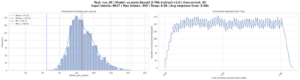
The left subplot in Figure 2 reveals the performance distribution pattern. A narrow, tall peak indicates consistent performance, while a wide, flatter distribution suggests variable performance. The vertical reference lines help quickly identify key statistics:

• Mean (red): Average performance
• Median (black): Middle value, less affected by outliers than the mean
• Min (blue): Worst-case performance
• Max (orange): Best-case performance

The right subplot tracks concurrency over time, revealing how the system handled the load pattern. This helps identify whether the test achieved the intended concurrency levels and maintained them throughout the test duration.

Comparative Analysis Across Test Runs

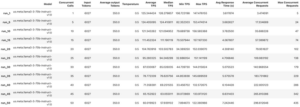
For comprehensive analysis across multiple test runs, we use an enhanced function that generates consolidated reports:

def create_all_plots_and_summary(df_dict, calls_dict, time_freq=’30S’):

# Calculate global min/max for consistent plotting

global_min, global_max = get_min_max_tokens_per_second(*df_dict.values())

 

# Generate visualizations and compile summary statistics

summary_stats = {}

 

for run_name in df_dict.keys():

# Extract metrics and create visualizations

# …

 

# Calculate concurrency metrics from events

# …

 

# Collect summary statistics

summary_stats[run_name] = {

‘Model’: model_id,

‘Concurrent Calls’: int(num_concurrent),

‘Input Tokens’: input_tokens,

‘Average output Tokens’: df[‘output_tokens’].mean(),

‘Temperature’: temperature,

‘Average TPS’: df[‘tokens_per_second’].mean(),

‘Median TPS’: df[‘tokens_per_second’].median(),

‘Min TPS’: df[‘tokens_per_second’].min(),

‘Max TPS’: df[‘tokens_per_second’].max(),

‘Avg Response Time (s)’: avg_ttlt,

‘Average Concurrent Requests’: avg_concurrency,

‘Max Concurrent Requests’: max_concurrency

}

 

# Create summary dataframe

summary_df = pd.DataFrame.from_dict(summary_stats, orient=’index’)

 

return figures, summary_df

This function generates both individual visualizations for each test run and a summary table that allows easy comparison across different concurrency levels. The summary table becomes particularly valuable when optimizing for specific metrics like average tokens-per-second or response time (see Figure 3).

 

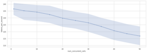
Performance Scaling Trend Analysis

To visualize the relationship between concurrency levels and performance metrics, we create statistical line plots with confidence intervals. These plots reveal both the central tendency and the variability of performance as concurrency increases (see Figure 4).

# Set a nice style

sns.set(style=”whitegrid”)

 

# Create statistical plots with advanced features

sns.lineplot(data=df,

x=”num_concurrent_calls”,

y=”tokens_per_second”,

marker=”o”,

estimator=”median”,

errorbar=(“pi”, 50))

Test Results and Analysis

With our methodology and metrics established, we can now examine actual performance data from AWS Bedrock models. This section presents detailed findings from our tests using the LLaMA 3.3 70B Instruct model, revealing important patterns in how the model scales with concurrent requests. These insights go beyond raw numbers to identify optimal operating points and potential bottlenecks.

For our tests with Llama 3 on AWS Bedrock, we used the following configuration:

model_id=”us.meta.llama3-3-70b-instruct-v1:0″

max_tokens=350

temperature=0.5

performance=”standard”

max_pool_connections = 20000

region_name = “us-west-2”

We used a simple philosophical prompt for our testing: “What is the meaning of life?”

Single Request Performance Baseline

Let’s first examine the performance of a single request to establish our baseline:

{‘response_text’: “The question of the meaning of life…”,

‘input_tokens’: 43,

‘output_tokens’: 350,

‘time_to_first_token’: 0.38360680200275965,

‘time_to_last_token’: 2.9637207640043925,

‘time_per_output_token’: 0.007392876681953103,

‘model_id’: ‘us.meta.llama3-3-70b-instruct-v1:0’,

‘provider’: ‘Bedrock:us-west-2’}

From this single invocation, we can extract several key performance metrics:

• Time to First Token (TTFT): ~0.38 seconds – This measures initial response latency
• Time to Last Token (TTLT): ~2.96 seconds – This measures total response time
• Time per Output Token: ~0.0074 seconds – How long it takes to generate each token
• Tokens per Second: ~135 tokens/second (calculated as 1/0.007392) – Raw generation speed

These baseline metrics represent optimal performance under no concurrent load and serve as our reference point for evaluating how performance changes under increasing concurrency.

Scaling with Concurrency

To comprehensively evaluate how performance scales with concurrency, we test a wide range of concurrency levels from 1 to 50 concurrent requests. For each level, we run 60 test iterations to ensure statistical significance of our results:

calls = [1, 5, 10, 15, 20, 25, 30, 35, 40, 45, 50]

# Run tests for num_calls

for num_calls in calls:

# Run 60 requests at each concurrency level

df_run, df_calls = await run_all_tests(

chat=my_chat,

prompt=my_prompt,

n_runs=60,

num_calls=num_calls,

use_logger=False,

schedule_mode=”interval”,

batch_interval=1.0

)

After collecting data across all concurrency levels, we observed a wide range of performance:

Minimum tokens_per_second: 9.23

Maximum tokens_per_second: 187.30

This significant range from ~9 to ~187 tokens-per-second demonstrates how dramatically performance can vary under different load conditions.

The graph in Figure 5 shows the relationship between concurrency level (x-axis) and tokens-per-second (y-axis), with the blue line representing median performance and the shaded area showing the 50% confidence interval. This visualization reveals several key patterns:

• Performance Degradation with Increased Concurrency: The line shows a clear downward trend, indicating that individual request performance (tokens-per-second) gradually decreases as concurrency increases.
• Per-Request Efficiency: At concurrency level 1, the median tokens-per-second is approximately 136, decreasing to about 117 at concurrency level 50 — a performance reduction of about 14%.
• Widening Variance: The confidence interval (shaded area) widens slightly at higher concurrency levels, suggesting more variable performance as the system handles more simultaneous requests.

When we combine this per-request performance data with the fact that throughput equals per-request performance multiplied by concurrency, we can derive total system throughput:

• At concurrency 1: ~136 tokens/second total throughput
• At concurrency 10: ~134 tokens/second per request × 10 requests = ~1,340 tokens/second total
• At concurrency 30: ~126 tokens/second per request × 30 requests = ~3,780 tokens/second total
• At concurrency 50: ~117 tokens/second per request × 50 requests = ~5,850 tokens/second total

This analysis reveals that while individual request performance decreases with concurrency, the total system throughput continues to increase, though with diminishing returns at higher concurrency levels.

For user experience considerations, the TTFT (responsiveness) pattern is particularly interesting. The graph in Figure 6 shows that TTFT actually remains remarkably stable across most concurrency levels, contrary to what might be expected:

• At concurrency 1-30: TTFT stays consistently around 0.28-0.29 seconds with minimal variation
• At concurrency 30-40: TTFT begins a slight but noticeable upward trend
• At concurrency 40-50: TTFT increases more significantly, reaching approximately 0.33 seconds at concurrency level 50

This represents only about a 17% increase in initial response time from concurrency level 1 to 50, which is surprisingly efficient. The widening confidence interval at higher concurrency levels indicates greater variability in TTFT, suggesting that while the median performance remains relatively good, some requests may experience more significant delays.

Impact of Large Prompts on Performance

To better understand how input size affects performance characteristics, we conducted a second set of experiments using a significantly larger prompt—a detailed creative writing framework for generating an epic fantasy narrative. This prompt weighed in at 6,027 tokens, compared to just 43 tokens in our initial prompt.

Here’s the baseline performance for a single request with this large prompt:

{‘response_text’: ‘This prompt is a comprehensive and detailed guide for generating an epic narrative titled “The Chronicles of Eldrath: A Saga of Light and Shadow.”…’,

‘input_tokens’: 6027,

‘output_tokens’: 350,

‘time_to_first_token’: 0.9201213920023292,

‘time_to_last_token’: 3.2595945539942477,

‘time_per_output_token’: 0.006703361495678849,

‘model_id’: ‘us.meta.llama3-3-70b-instruct-v1:0’,

‘provider’: ‘Bedrock:us-west-2’}

Key observations from the single large-prompt request:

• TTFT increased dramaticallyto ~0.92 seconds (compared to ~0.38 with the small prompt)
• TTLT increased moderatelyto ~3.26 seconds (compared to ~2.96 with the small prompt)
• Tokens per second actually improved slightlyto ~149 (calculated as 1/0.006703)

This slight improvement in token generation speed with larger prompts at low concurrency levels is interesting but could likely be attributed to natural service variability rather than representing a consistent performance advantage. What’s more significant is how these performance characteristics change under increasing concurrency, where we see clear and substantial divergence between small and large prompts.

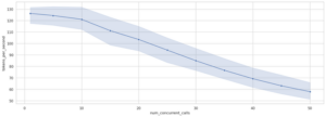
When scaling concurrency with the large prompt, the pattern changes significantly, as shown in Figure 7:

• Much steeper degradation curve: The tokens-per-second metric drops from a median of ~126 at concurrency level 1 to ~58 at concurrency level 50—a reduction of over 50%, compared to only 14% with the small prompt.
• Lower overall performance: At concurrency level 50, the median tokens-per-second is only ~58, with some requests dropping as low as ~8 tokens-per-second.

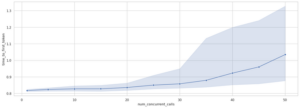
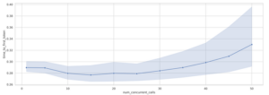
Looking specifically at the TTFT behavior with the large prompt, the newly provided graph (Figure 8) reveals a much more pronounced pattern of degradation compared to the small prompt:

• At concurrency 1-30: TTFT remains relatively stable around 0.82-0.86 seconds
• At concurrency 30-40: TTFT begins to rise more steeply, reaching about 0.92 seconds
• At concurrency 40-50: TTFT accelerates dramatically upward to over 1.03 seconds

Most notably, the confidence interval widens significantly at higher concurrency levels, with the upper bound exceeding 1.3 seconds at concurrency level 50. This indicates that while median TTFT increases by about 25% from levels 1 to 50, some users may experience initial response delays that are more than 50% longer than baseline.

This degradation profile for TTFT with large prompts is substantially different from what we observed with small prompts, where TTFT remained relatively stable until much higher concurrency levels. The earlier and steeper degradation suggests that AWS Bedrock prioritizes different aspects of performance when dealing with large input contexts under load.

When analyzing the concurrency level of 50 in more detail (Figure 8), the histogram of tokens-per-second shows:

• Mean: 60.02 tokens/second
• Median: 57.94 tokens/second
• Min: 7.89 tokens/second
• Max: 122.38 tokens/second

This represents a much more significant performance impact than observed with the small prompt, demonstrating that large input contexts not only increase initial latency but also reduce the system’s ability to efficiently manage concurrent requests.

When calculating total system throughput with the large prompt:

• At concurrency 1: ~126 tokens/second total throughput
• At concurrency 10: ~121 tokens/second per request × 10 requests = ~1,210 tokens/second total
• At concurrency 30: ~85 tokens/second per request × 30 requests = ~2,550 tokens/second total
• At concurrency 50: ~58 tokens/second per request × 50 requests = ~2,900 tokens/second total

This shows diminishing returns setting in much earlier—the system achieves only minimal throughput gains beyond concurrency level 30. The right side of Figure 8 illustrates the actual concurrency achieved during the test, showing fluctuations between 250-400 concurrent requests as the system processes the workload.

Comparison of System Throughput: Small vs. Large Prompts

When comparing the total system throughput between small and large prompts across different concurrency levels, we observe striking differences in scaling patterns:

Concurrency Level	Small Prompt Throughput	Large Prompt Throughput	Difference (%)
1	~136 tokens/sec	~126 tokens/sec	-7.4%
10	~1,340 tokens/sec	~1,210 tokens/sec	-9.7%
30	~3,780 tokens/sec	~2,550 tokens/sec	-32.5%
50	~5,850 tokens/sec	~2,900 tokens/sec	-50.4%

At low concurrency levels (1-10), the difference in total system throughput is relatively small—only about 7-10% lower with large prompts. However, this gap widens dramatically as concurrency increases. At concurrency level 30, the large prompt system achieves only about two-thirds the throughput of the small prompt system. By concurrency level 50, the difference becomes even more pronounced, with the large prompt system delivering just half the throughput of the small prompt system.

This comparison reveals several key insights:

• Different scaling curves: Small prompts exhibit near-linear scaling up to concurrency level 50, while large prompts show severely diminishing returns after concurrency level 30.
• System bottlenecks emerge earlier with large prompts: The sharp drop-off in throughput gains suggests that processing large input contexts creates resource bottlenecks that aren’t as significant with smaller inputs.
• Optimal concurrency points differ: For small prompts, increasing concurrency to 50 or potentially higher still yields significant throughput benefits. For large prompts, the optimal concurrency point appears to be around 30-35, after which additional concurrent requests provide minimal throughput benefits while degrading individual request performance.

Conclusion: Translating Performance Insights into Practical Applications

The performance testing approach outlined in this blog provides valuable insights into how AWS Bedrock foundational models behave under various load conditions. By systematically measuring key metrics like tokens-per-second, response times, and concurrency impacts, we’ve established a comprehensive understanding that can directly inform production implementations.

Key Takeaways

• Service Quota Implications Are Significant:All results in our testing were calculated using special elevated service quotas that were granted specifically for testing with LLaMA 3.3 70B Instruct on Bedrock. These enhanced quotas of 6,000 RPM and 36 million TPM were substantially higher than the default values of 800 RPM and 600,000 TPM available to standard AWS accounts. This special allocation was necessary to thoroughly explore performance at high concurrency levels, and is not representative of what most customers will initially have access to. This dramatic difference underscores the critical importance of understanding your specific quota allocations and planning for quota increase requests well in advance when designing scalable LLM applications.
• Input Size Significantly Impacts Scaling:As demonstrated in our tests with LLaMA 3.3, large prompts (6,000+ tokens) scale very differently from small prompts. While small prompts maintain relatively linear throughput scaling up to concurrency level 50, large prompts experience dramatic performance degradation beyond concurrency level 30.
• Response Time Characteristics Vary:Time to First Token (TTFT) remains remarkably stable for small prompts even under high load, but degrades much more severely with large prompts. This has direct implications for user experience design and capacity planning.
• Optimal Concurrency Points Differ by Use Case:Applications using smaller prompts can benefit from higher concurrency levels (40-50+), while those with large prompts should consider limiting concurrency to around 30-35 to maintain acceptable performance.

Service Quota Management

The default AWS Bedrock quotas (800 RPM and 600,000 TPM) would significantly constrain the scalability demonstrated in our tests. Our testing utilized specially granted elevated quotas of 6,000 RPM and 36 million TPM, which required formal justification and are not automatically available to AWS customers. Without these special allocations, the maximum achievable concurrency would be considerably lower. This highlights why quota management is not merely an operational concern but a fundamental architectural consideration that should be addressed early in your application design process.

When planning for quota increases, it’s essential to understand that the relationship between quota limits and actual performance isn’t always straightforward. Assuming a linear correspondence between concurrent requests and token throughput (which, as seen in the blog, is not always true depending on prompt size), higher quotas should theoretically allow for proportionally more concurrent requests. However, our testing revealed that performance begins to degrade non-linearly with large prompts beyond certain concurrency thresholds, meaning that simply increasing these quotas may not yield proportional performance improvements in all scenarios.

This last point is based on observed patterns and remains somewhat speculative, as we don’t have visibility into exactly how the AWS Bedrock infrastructure manages these scenarios behind the scenes or how resources are allocated across different request patterns at scale.

By conducting similar performance testing with your actual prompts and response patterns, you can:

• Calculate your true capacity requirements based on expected usage patterns
• Determine optimal concurrency levels for your specific workflows
• Support quota increase applications with concrete performance data that justifies your specific resource needs

Implementation Recommendations

• Request appropriate quota increases early in your project lifecycle – default quotas may not be sufficient for many production workloads
• For applications with large input contexts, limit how many requests can run at the same time to maintain good performance
• Keep track of both typical response times and slowest response times (p95, p99) to make sure all users have a good experience, not just the average user

Performance testing connects abstract quota values to real-world capacity planning. Through systematic measurement and analysis of model performance under various conditions, you’ll gain insights that can inform decisions, capacity planning, and quota management—ultimately leading to more efficient and effective LLM implementations.

Get the Code

The complete implementation of the testing framework discussed in this blog is available on GitHub:

The repository contains the full Python codebase, visualization utilities, and example notebooks to guide you in conducting your own performance tests using AWS Bedrock foundation models.